The Poisson Distribution: Modeling Rare Events at a Known Rate

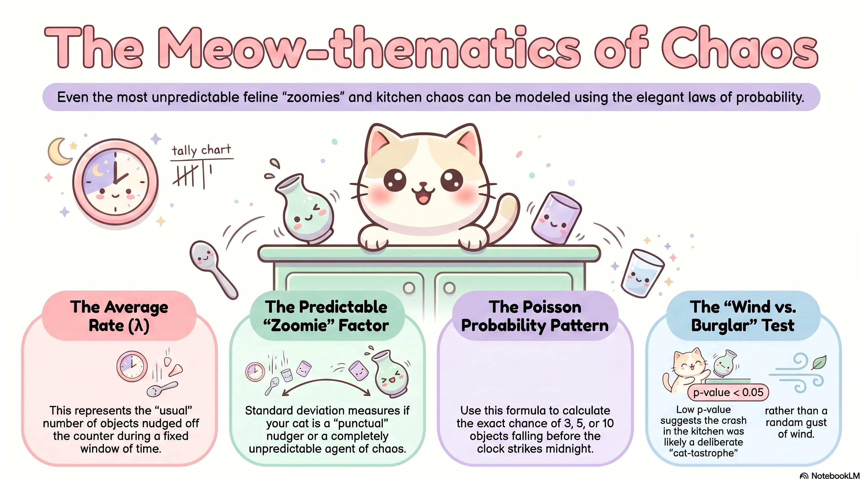
At some point each evening, a cat will knock something off a surface. Not always the same thing. Not at any predictable moment. But at a rate that, if you tracked it long enough, would settle into something stable. Three objects per evening, roughly. Some nights zero. Some nights five. Never a fraction.

The Poisson distribution was built for exactly this situation.

What It Models

The Poisson distribution counts the number of events occurring in a fixed interval of time or space when the events happen independently, at a constant average rate, and cannot occur simultaneously. The interval can be an evening, a square kilometer, or a page of text. The events can be falling objects, radioactive decays, or typographical errors.

The distribution has a single parameter, $\lambda$ (lambda), which represents the expected number of events in the interval. Everything follows from $\lambda$.

The PMF

The probability of observing exactly $k$ events is:

$$P(X = k) = \frac{\lambda^k e^{-\lambda}}{k!}, \quad k = 0, 1, 2, \ldots$$

The factor $\lambda^k / k!$ comes from the Taylor expansion of $e^\lambda$. The $e^{-\lambda}$ term is the normalizing constant that ensures all probabilities sum to one. Together they produce a distribution defined over all non-negative integers, with no upper bound on $k$.

One useful quantity to internalize: $P(X = 0) = e^{-\lambda}$. The probability of zero events decreases exponentially as the rate increases. At $\lambda = 3$, there is about a 5% chance of a quiet evening.

A Worked Example

Assume a cat averages three shelf-clearing incidents per evening, and that these occur independently with no tendency to cluster. We model $X \sim \text{Poisson}(3)$.

The probability of exactly two incidents:

$$P(X = 2) = \frac{3^2 e^{-3}}{2!} = \frac{9 \times 0.0498}{2} \approx 0.224$$

The probability of four or more:

$$P(X \geq 4) = 1 - P(X \leq 3) = 1 - \sum_{k=0}^{3} \frac{3^k e^{-3}}{k!} \approx 0.353$$

On roughly one in three evenings, the cat exceeds her average.

Mean and Variance

The Poisson distribution has a distinctive property: its mean and variance are both equal to $\lambda$.

$$E[X] = \lambda \qquad \text{Var}(X) = \lambda$$

This is not a coincidence of the formula. It reflects the structure of the underlying process. When events occur independently at a constant rate, the spread of the count around its mean grows at the same rate as the mean itself.

This equality is also diagnostically useful. If you observe a count variable whose sample mean and sample variance are approximately equal, the Poisson model is worth considering. If the sample variance substantially exceeds the mean -- a condition called overdispersion -- the Poisson model is likely inadequate.

Where It Comes From

The Poisson distribution can be derived as a limiting case of the binomial. Suppose you run $n$ trials with success probability $p = \lambda / n$, and then let $n \to \infty$ while holding $\lambda = npfixed. As $n grows, the binomial PMF converges to the Poisson PMF.

This is not just mathematical trivia. It explains when the Poisson is the right model: when events are rare relative to the number of opportunities, and the count of opportunities is large enough that it no longer meaningfully constrains the outcome. The actual $n$ becomes irrelevant. Only the rate $\lambda$ survives.

The Poisson Process

The Poisson distribution is the marginal distribution of a more general object: the Poisson process, a model for events occurring continuously in time. In a Poisson process, the number of events in any interval of length $t$ follows a Poisson distribution with parameter $\lambda t$, where $\lambda$ is now the rate per unit time. Events in non-overlapping intervals are independent.

The practical consequence: if you know the rate per hour, you can compute the distribution over any time window by scaling $\lambda$ accordingly. The structure is preserved under that rescaling, which makes the Poisson process unusually flexible.

Assumptions and Violations

The Poisson model requires independence and a constant rate. Both assumptions can fail.

Events that cluster -- where one occurrence makes another more likely -- produce overdispersion. Events that deplete a finite resource, or that have an underlying rhythm (a cat that knocks things over when hungry, and is hungry on a schedule), violate the constant-rate assumption.

When these violations are mild, the Poisson is often a reasonable approximation. When they are severe, the negative binomial distribution is a common alternative: it allows the variance to exceed the mean, and reduces to the Poisson as a special case.

The model is not fragile, but it is not unconditional. Like all probability distributions, it is a description of a mechanism. Whether that mechanism matches the system you are studying is a question about the world, not about the mathematics.