The Binomial Distribution: Counting Successes in Fixed Trials

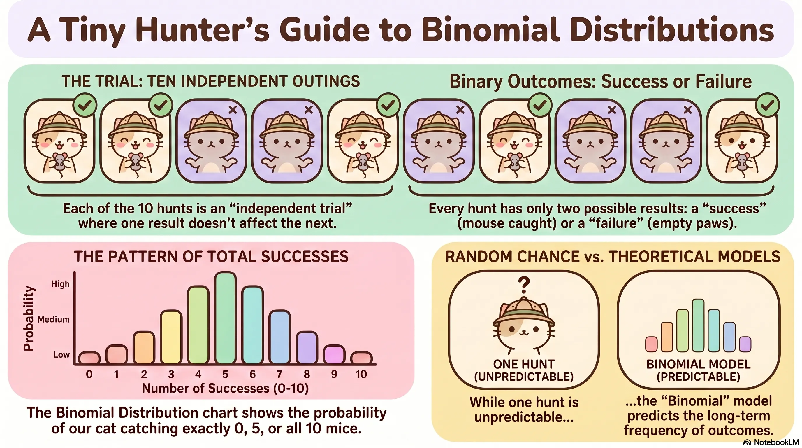
A cat that hunts is running an experiment, whether she knows it or not. Each pounce is a trial. It either succeeds or it does not. The outcome of one attempt does not influence the next. And if you watch long enough, you start asking a different question: not whether she catches something, but how many she catches in a given session.

That is the question the binomial distribution answers.

The Setup

The binomial distribution applies when four conditions hold. There are exactly $n$ trials. Each trial results in one of two outcomes, conventionally called success and failure. The trials are independent. And the probability of success, $p$, is the same on every trial.

These four conditions define a sequence of Bernoulli trials, named for the Swiss mathematician Jacob Bernoulli. A single Bernoulli trial is just a coin flip with a possibly unfair coin. The binomial distribution describes what happens when you run $n$ of them and count the successes.

Call that count $X$. The random variable $X$ can take any integer value from $0$ to $n$.

The PMF

The Probability Mass Function gives the probability of exactly $k$ successes:

$$P(X = k) = \binom{n}{k} p^k (1-p)^{n-k}$$

The formula has two parts, and both matter.

The term $p^k (1-p)^{n-k}$ is the probability of one specific sequence containing exactly $k$ successes and $n - k$ failures. If $k = 3$ and $n = 5$, for instance, one such sequence is success-success-success-failure-failure, with probability $p^3 (1-p)^2$.

But there are many sequences with exactly three successes. The binomial coefficient $\binom{n}{k}$, read as "$n$ choose $k$," counts how many:

$$\binom{n}{k} = \frac{n!}{k!\,(n-k)!}$$

Multiply the two pieces together and you have the probability of getting $k$ successes in any order. The formula is not arbitrary. It follows directly from counting.

A Worked Example

Suppose a cat succeeds on roughly 30% of pounce attempts, and makes eight attempts in a session. Each attempt is independent. We want $P(X = 3)$: the probability of exactly three successes.

$$P(X = 3) = \binom{8}{3}(0.3)^3(0.7)^5$$

$$= 56 \times 0.027 \times 0.16807 \approx 0.254$$

About a 25% chance of exactly three successes. The distribution also gives us the full picture: we can compute $P(X = 0)$ through $P(X = 8)$, and all eight values sum to one.

Expected Value and Variance

The expected number of successes is:

$$E[X] = np$$

For our hunting cat, that is $8 \times 0.3 = 2.4$ successes per session. Not a whole number, which is fine -- expected value is not a prediction of any single outcome. It is the long-run average.

The variance is:

$$\text{Var}(X) = np(1-p)$$

And the standard deviation is $\sqrt{np(1-p)}$. Both depend on $p$ in a way worth noting: the variance is largest when $p = 0.5$ and shrinks toward zero as $p$ approaches either extreme. When success is nearly certain or nearly impossible, there is little variability -- you already know roughly what will happen.

Assumptions and When They Break

The binomial model is exact when the four conditions are exactly met. In practice, they rarely are. What matters is how badly they are violated.

Independence is the most commonly broken condition. Whether one hunting attempt affects the next depends on the prey behavior, the cat's fatigue, and a dozen other things. If trials influence each other, the binomial is at best an approximation.

The fixed-$p$ assumption can also fail. A cat may improve over the course of a session, or tire. If $p$ drifts, the binomial is still sometimes useful as a baseline, but it will misrepresent the tails of the distribution.

The Normal Approximation

For large $n$, the binomial distribution is well-approximated by a normal distribution with mean $np$ and standard deviation $\sqrt{np(1-p)}$. The approximation is reliable when $np \geq 5$ and $n(1-p) \geq 5$. Outside that range, the exact binomial is preferable.

The binomial probability calculator computes exact values for any $n$, $p$, and $k$ using log-space arithmetic to handle large $n$ without numerical underflow.

What Makes It Useful

The binomial distribution is not especially subtle, but its simplicity is the point. When the four conditions hold -- or approximately hold -- it is the right model, and it is completely tractable. You can compute the PMF, the CDF, the expected value, and the variance in closed form.

The harder question is always whether the conditions hold. The binomial distribution gives the right answer to the right question. Identifying the right question first is the more consequential step.